Note: this is general educational material about quantitative research practice. It is not investment advice, and it describes no real strategy, no real data, and no real trading results. Every simulation below is a toy written to demonstrate a mechanism — synthetic data, deliberately exaggerated magnitudes, illustrative numbers throughout.
Why backtests lie to their own authors
A backtest is a claim about the past made by someone who already knows how the past turned out. That asymmetry — the researcher knows the future relative to every bar in the data — is the root of nearly every backtesting failure. The question is never “does the strategy work on history?” but “does the history actually test the strategy?” Most of the time, quietly, it does not.
The lies a backtest tells are rarely deliberate. They creep in through data quirks, through convenience shortcuts in the simulation, and through the sheer number of ideas tried before the “final” one. Each is individually small. Together they compound into strategies that look brilliant in-sample and die on contact with live data.
Lookahead bias: knowing what you couldn’t have known
Lookahead bias is using information that was not available at the decision point. It is the single most common backtest flaw, and it hides everywhere:
- Point-in-time data. Financial statements, economic indicators, and even price data get revised. A backtest fed on current-vintage fundamentals is simulating trades on earnings numbers that didn’t exist yet in their present form.
- Rebalancing and corporate actions. Index membership, stock splits, delistings — using today’s constituent list to build yesterday’s portfolio silently drops every company that failed.
- Signal computation order. Computing a “daily close” signal and trading on it at the close assumes you can transact at the price you just observed. In practice the signal only exists after the bar completes.
The fix is mechanical discipline: every input to the simulation must be point-in-time correct, and every signal must be lagged by its real-world latency. If you can’t document the exact timestamp at which each piece of data was knowable, you don’t have a backtest — you have a fantasy.
The classic one-line version of the bug, and the fix, in pandas. The signal here is pure noise — which is exactly what makes the demonstration work:
import numpy as np
import pandas as pd

# --- Synthetic setup: one year of daily bars, pure random walk (illustrative) ---
rng = np.random.default_rng(7)
close = 100.0 * np.exp(np.cumsum(rng.normal(0.0004, 0.01, size=252)))

sig = pd.Series(close).pct_change()   # "signal": today's move, known only AFTER the close
ret = sig.copy()                      # close-to-close return on the same bar

# WRONG: trade AT the close on the close-t signal. P&L = |r_t| -- always >= 0,
# so even pure noise manufactures edge. This is the leak, in one line.
pnl_leaky = (np.sign(sig) * ret).dropna()

# RIGHT: a signal observed at close t becomes a position for bar t+1.
pnl_honest = (np.sign(sig.shift(1)) * ret.shift(-1)).dropna()

def sharpe(p):
    return p.mean() / p.std() * np.sqrt(252)

print(f"leaky  Sharpe (illustrative): {sharpe(pnl_leaky):.2f}")
print(f"honest Sharpe (illustrative): {sharpe(pnl_honest):.2f}")
On noise, the honest version hovers near zero while the leaky version prints a spectacular Sharpe — not because the signal has edge, but because the simulation let the strategy trade on information it could not have had. Any time a backtest’s edge looks too clean, the first question is whether the signal was shifted.
Survivorship bias: the graveyard the data forgot
Most commercial datasets cover securities that exist now. The companies that went bankrupt, got acquired, or were delisted quietly vanish from the universe. A backtest over the survivors inherits their success: it never holds the stock that went to zero because that stock isn’t in the data.
The practical consequence is an upward bias in historical returns that looks exactly like alpha. The defense is a survivorship-bias-free dataset — one that includes delisted securities with their full histories — or at minimum an honest estimate of the bias’s magnitude applied as a haircut to reported performance. I work through both biases end to end, with runnable toy simulations, in Survivorship Bias and Lookahead: Two Backtest Killers, with Code.
Transaction costs and slippage: the tax reality imposes
Many a strategy dies not on bad signals but on arithmetic. Backtests that ignore or understate costs are the quantitative equivalent of budgeting without taxes.
- Commissions and fees. Small per-trade, decisive at high turnover.
- Slippage. The difference between the simulated fill and the actual fill, driven by latency, market impact, and the spread. Assume the conservative side of any uncertainty.
- Market impact. A strategy that “works” trading 1% of average daily volume is a different strategy than one trading 20% of it. Size the simulation to the capital the strategy can actually absorb.
- Borrow costs and financing. Short legs pay borrow; leveraged legs pay financing. Both vary with the very conditions the strategy trades through.
A useful discipline: compute the strategy’s break-even cost per trade — the round-trip cost at which the edge disappears. If realistic slippage estimates land anywhere near that number, there is no edge to validate:
# --- Cost-aware P&L on the honest toy signal (illustrative costs) ---
pos = np.sign(np.concatenate([[0.0], np.diff(close)])[:-1])  # yesterday's move, tradable today
ret = np.diff(close) / close[:-1]
pnl = pos * ret                                             # honest: position known before return
turnover = np.abs(np.diff(pos, prepend=pos[0])) / 2          # 1.0 on every flip
cost_bp = 8.0                                               # illustrative round-trip cost, basis points

pnl_costed = pnl - turnover * cost_bp / 1e4
print(f"illustrative gross Sharpe: {pnl.mean()/pnl.std()*np.sqrt(252):.2f}")
print(f"illustrative net   Sharpe: {pnl_costed.mean()/pnl_costed.std()*np.sqrt(252):.2f}")

flips = turnover.sum()
print(f"illustrative break-even round-trip cost: {pnl.sum()/max(flips,1)*1e4:.1f} bps")
Note what this does to research behavior: once every candidate strategy must clear its break-even cost under conservative assumptions, most candidates die in the notebook — which is where you want them to die.
Overfitting: the optimizer finds luck, not edge
Given enough trials, any dataset will surrender a strategy with a beautiful equity curve. This is data dredging wearing a lab coat: try a hundred parameter combinations, keep the best, report its backtest as though it were the first and only idea. The reported Sharpe ratio is then the maximum of a hundred draws from a distribution of noise — a statistic virtually guaranteed to flatter.
The defense is to adjust for the number of trials. The deflated Sharpe ratio (Bailey and López de Prado) answers the question “is this Sharpe exceptional, or is it what you’d expect as the best of K tries under the null of no edge?” — computing the expected best Sharpe under the null and testing whether the reported one clears it:
import numpy as np
from scipy.stats import norm

# --- Deflated Sharpe ratio (Bailey & López de Prado), illustrative inputs ---
K = 200              # strategy variants tried during research (illustrative)
T = 252              # backtest length in bars
sr_reported = 1.8    # best Sharpe among the K trials (illustrative)
sr_trials = np.random.default_rng(0).normal(0.0, 0.5, size=K)  # all K trial Sharpes
gamma = 0.5772156649
gamma3, gamma4 = 0.0, 3.0   # return skew / kurtosis (illustrative: Gaussian)

V = sr_trials.var()
sr0 = np.sqrt(V) * ((1 - gamma) * norm.ppf(1 - 1/K)
                    + gamma * norm.ppf(1 - 1/(K * np.e)))       # expected best under the null
denom = np.sqrt(max((1 - gamma3*sr_reported + (gamma4-1)/4*sr_reported**2) / T, 1e-12))
dsr = norm.cdf((sr_reported - sr0) / denom)

print(f"reported Sharpe {sr_reported:.2f} over {K} trials "
      f"-> expected best under null {sr0:.2f}, deflated Sharpe ratio {dsr:.2f}")
The deeper fix is procedural: reduce the researcher’s degrees of freedom before seeing the data. Keep a trial log — every variant tried, not just the winner — because the trial count K is the input the correction needs, and researchers who don’t log it will misremember it downward. And prefer a strategy with a credible mechanism (a documented market friction, a risk premium, a structural asymmetry) that backtests modestly over one with no story and a spectacular equity curve. The story is the prior; the backtest updates it.
Walk-forward validation: judge only the out-of-sample segments
A single in-sample fit proves a strategy can memorize. Walk-forward analysis replaces the single fit with a rolling discipline: fit (or select parameters) on an in-sample window, evaluate on the next out-of-sample window, roll forward, repeat. The in-sample segments are training loss — reported for transparency, never as a performance claim. Only the concatenated out-of-sample segments count:
# --- Rolling walk-forward on the toy signal (illustrative) ---
train, step = 126, 63
oos_segments = []
for start in range(0, len(close) - train, step):
    tr = slice(start, start + train)                 # in-sample: fit here
    te = slice(start + train, start + train + step)  # out-of-sample: judged here
    oos_segments.append((pos[te] * ret[te]).mean())  # the rule has no parameters; a real
                                                     # strategy would fit them on `tr`

print("illustrative out-of-sample segment means:", np.round(oos_segments, 5))
print("report the OOS column. Flat OOS is a finding, not a failure.")
Two refinements matter when labels overlap window boundaries. Purged k-fold drops training samples whose label windows touch the test block (a forward-looking return label computed near the fold boundary peeks into the test set). Embargo adds a fixed gap after each test block, because serial dependence doesn’t stop exactly at the boundary you drew:
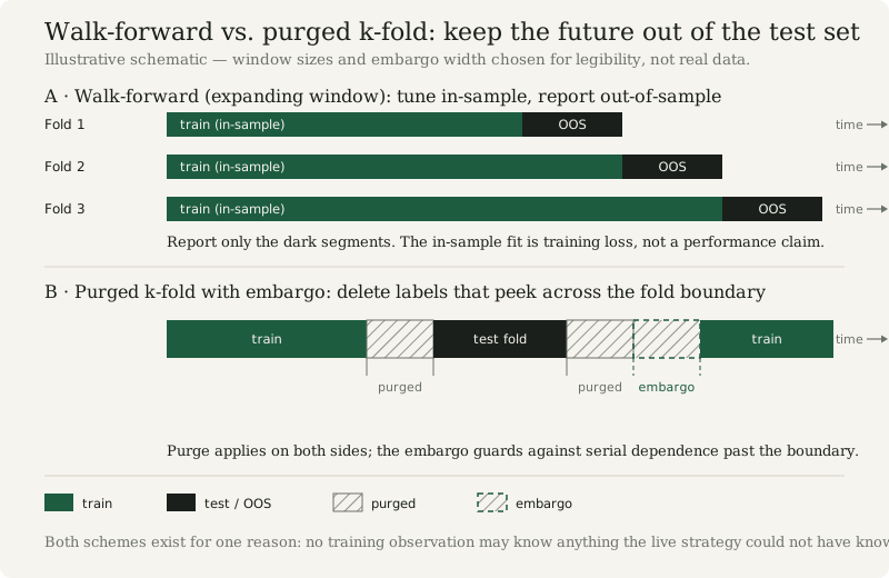
Figure — walk-forward tunes in-sample and reports only the dark out-of-sample segments; purged k-fold removes training samples whose labels overlap the test block and adds an embargo gap. Schematic, not real data.
And keep one period truly locked away: a final holdout that no optimization and no ad-hoc tweaking ever touches. The strategy is what survives that window untouched. If the holdout is consulted even once to “check” a parameter choice, it is no longer a holdout — it is another training set with better PR.
A validation checklist
Before trusting a backtest, run it through this gauntlet:
- Point-in-time audit. Every input timestamped, every signal lagged by real latency.
- Survivorship check. Dataset includes delisted securities, or bias is estimated and applied.
- Trial accounting. Every variant tried is logged; reported metrics are adjusted for multiple testing.
- Walk-forward results. Out-of-sample segments reported separately and honestly — flat is a finding, not a failure.
- Cost sensitivity. Results survive conservative slippage and impact assumptions, not just the base case.
- Regime robustness. The strategy holds up across distinct market regimes in the data (crises, calm periods, rate cycles), not just the average.
- Implementation audit. The simulated fills, sizing, and constraints match what operations can actually execute.
A backtest that passes this checklist is still not proof — proof only comes from live trading. But it is an honest hypothesis, and honest hypotheses are the raw material everything downstream depends on.