This article is a practitioner’s playbook for model validation in the spirit of SR 11-7, the US Federal Reserve’s guidance on model risk management. It uses a clinical risk-scoring setting — like my public cardiac-surgery-predictive-model project — as a running illustrative example. All code is illustrative reconstruction, not production or verbatim repo code.
Most model validation I’ve seen is a confirmation ritual: train, report a good metric, ship. SR 11-7 — the Federal Reserve’s supervisory guidance on model risk management, written for banks but applicable anywhere a model’s output drives consequential decisions — demands the opposite posture. Validation is the organized attempt to kill the model. A model that survives honest attempts at destruction is the only kind worth deploying.
The guidance structures validation around three pillars, plus governance and documentation as the frame that holds them up:
- Conceptual soundness — is the model’s design, theory, and logic appropriate for its intended use?
- Ongoing monitoring — does it keep working once deployed, in a changing world?
- Outcomes analysis — do its predictions hold up against reality and against alternatives?
Governance (who owns the model, who can override it, who signs off) and documentation (enough detail that an independent reviewer can reproduce the validation) wrap the three pillars. This article is the applied companion: what each pillar looks like in practice, with code.
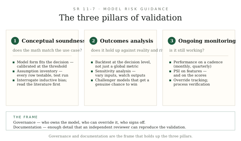
Figure — the three pillars of SR 11-7 validation, held up by governance and documentation.
Know the failure modes first
Before the pillars, memorize the five ways models fail validation. You will see every item in the wild:
- Leakage. The target, or a proxy of it, contaminates the features or the test set. The model looks brilliant and knows nothing.
- Evaluation theater. A test set drawn from the same distribution, time period, and collection process as training — measuring memorization, not generalization.
- Conceptual mismatch. A classifier solving a ranking problem, a point predictor where the decision needs a distribution, a model optimizing a metric nobody decided on.
- Brittleness. Performance that collapses under small distribution shifts the training data never contained.
- Decay without monitoring. A model approved on 2023 data quietly rotting as the world moves on.
A validation workflow exists to make each of these hard to miss, not just possible to find. The pillars below are organized to hunt them in the order that catches them cheapest.
Pillar 1: Conceptual soundness — does the math match the use case?
Conceptual soundness is the least glamorous and most skipped pillar. It asks: given what this model is for, are its choices defensible? A Gradient Boosting regressor predicting postoperative risk is conceptually sound only if the answers to a handful of questions hold up.
Does the model form fit the decision? A model that outputs a point estimate of risk, feeding a thresholded flag (“review this patient”), needs calibrated magnitudes at the threshold — not just good ranking. If the validation only reports a global fit metric, the conceptual link between what was optimized and what the decision needs is broken. (This is the R² trap in full: optimizing explained variance when the decision needs calibrated tail probabilities.)
Is the data representative of the use population? A model trained on elective-procedure patients and applied to emergency cases is not validated — it’s extrapolated. Representativeness covers the feature distributions, the outcome base rates, and the data-generating process: were the predictors actually available before the outcome, as they will be at decision time? Leakage isn’t just a modeling bug; it’s a conceptual-soundness failure, because the model was validated against information the deployment will never have.
What are the assumptions, and what breaks if they’re wrong? Every model is a bundle of assumptions wearing a trench coat. Write them down. Here’s the inventory format I use — one row per assumption, with the test that would falsify it:
| Assumption | Why it matters | How to test it | What breaks if wrong |
|---|---|---|---|
| Predictors are measured before the outcome, as at decision time | Leakage inflates validation metrics | Audit feature timestamps vs. outcome timestamps | All performance numbers are fiction |
| Training population matches deployment population | Model extrapolates poorly outside its support | Compare feature/outcome distributions (see PSI below) | Calibration collapses on new cohorts |
| Outcome labels are correct and consistently defined | Supervised learning inherits label error | Adjudication sample re-labeling; inter-rater agreement | Model learns the labeling process, not the phenomenon |
| Missingness is ignorable after imputation | Imputation bakes in a missingness model | Compare performance on complete vs. imputed rows | Biased predictions for patients with sparse records |
| The decision threshold’s cost ratio is stable | Threshold optimality depends on costs | Sensitivity sweep over cost ratios | Optimal threshold drifts; flags misfire |
| Residual behavior is well-behaved (per transforms like Yeo-Johnson) | Intervals and tests assume residual structure | Residual-vs-fitted plots, QQ plots on held-out data | Confidence intervals mis-cover |
| No feedback loop: predictions don’t change future labels | Validation assumes i.i.d. future data | Track whether flagged cases receive interventions that alter outcomes | Backtests overstate value; model “works” by causing its own success |
The table is the deliverable. A validation report without an assumption inventory is a test report for a machine whose operating envelope was never specified. For each row, “how to test it” should point at an actual analysis in the report — or the row is decoration.
For ML models specifically, also interrogate the inductive bias: what patterns is this model class predisposed to find, and are those the patterns that actually drive the outcome? A gradient-boosted tree and a neural network can achieve identical test metrics while “believing” completely different things about the world — and only one of those beliefs may survive the deployment population.
Does the literature already know how this fails? The first move is embarrassingly unglamorous: read. Has this approach been tried before? What did the literature find — including the failures, which teach more than the successes? This isn’t academic gatekeeping; it’s base rates. If a class of models has historically broken under regime change, the validator’s job is to ask what makes this instance different — and to require evidence, not optimism, as the answer. A model built on a technique with known failure modes in this domain starts with a burden of proof, not a presumption of innocence.
When the math is right but the model is wrong. The dangerous models aren’t the ones with coding errors — those get caught. The dangerous ones are mathematically flawless implementations of the wrong idea: a precisely calibrated model of a relationship that no longer exists, an elegant optimizer for an objective nobody actually wants, a sophisticated ensemble that learned the data collection process instead of the phenomenon. No amount of backtesting catches this, because the backtest shares the same wrong idea. That’s why conceptual soundness comes first: it asks whether the model deserves to be tested, before testing dignifies it.
Developmental evidence — SR 11-7’s term for the paper trail — means the choices are documented with alternatives considered: why this algorithm, why these hyperparameters, what was tried and rejected. A reviewer should be able to reconstruct why, not just what.
Validate the data before the model
Data validation comes before model validation, because garbage data makes every downstream check meaningless:
- Schema and range checks. Types, bounds, missingness patterns, impossible values. Automate these; run them on every data refresh.
- Leakage detection. For each feature, ask: “could this value have been known at prediction time?” Check timestamps ruthlessly. Features computed over windows that include the target period are the classic killer.
- Split integrity. Verify the split actually separates what you think it separates — by time, by entity, by whatever dimension deployment will test. Check for duplicate or near-duplicate records straddling the split.
- Representativeness. Does the development data resemble the population the model will score? Sample bias here becomes performance bias in production.
Skip this section and everything below it — the backtests, the challenger, the PSI monitors — inherits whatever the data got wrong. Most “model failures” I’ve seen postmortems of trace back to one of these four checks being skipped, not to the algorithm.
Pillar 2: Outcomes analysis — does it hold up against reality and rivals?
Outcomes analysis compares model outputs to actual outcomes — backtesting — and to benchmarks. Three components:
Backtesting. On genuinely held-out data (out-of-time beats out-of-sample when the deployment faces time drift: train on 2023–2024, validate on 2025), compare predictions to realized outcomes. For a risk score, that means calibration in the tails, threshold-decision confusion matrices at the operating threshold, and interval coverage — not just a global metric. Backtest at the decision level: simulate the flag/review workflow and measure the outcomes that the decision was supposed to improve.
Sensitivity analysis. Vary the inputs and assumptions and watch the outputs. How much does the risk score move when a key predictor shifts by a plausible measurement error? Which features drive the largest prediction changes (permutation or SHAP-based, on held-out data)? If a single feature’s noise can flip a patient’s flag, the model is brittle regardless of its average metric — and the assumption-inventory row on measurement error just failed its test.
Challenger models. The single highest-value validation exercise: build at least one credible alternative — a simpler model (regularized linear), a different inductive bias (a tree model if the champion is linear, or vice versa) — and compare on the same held-out data, across multiple metrics. The challenger does two jobs: it checks whether the champion’s complexity is earning its keep, and it provides a fallback if the champion degrades. Here’s the comparison harness. It assumes a train/test split — a synthetic one to run it against:
# --- Synthetic setup: train/test split (illustrative stand-in) ---
from sklearn.datasets import make_regression
from sklearn.model_selection import train_test_split

X, y = make_regression(n_samples=2000, n_features=15, noise=10.0, random_state=42)
X_train, X_test, y_train, y_test = train_test_split(
    X, y, test_size=0.25, random_state=42
)
import numpy as np
from sklearn.linear_model import RidgeCV
from sklearn.ensemble import GradientBoostingRegressor
from sklearn.metrics import mean_absolute_error, mean_squared_error, r2_score

def evaluate(name, y_true, y_pred):
    return {
        "model": name,
        "R2": r2_score(y_true, y_pred),
        "MAE": mean_absolute_error(y_true, y_pred),
        "RMSE": np.sqrt(mean_squared_error(y_true, y_pred)),
    }

# champion vs. challenger, same held-out set, multiple metrics
champion_pred = GradientBoostingRegressor(random_state=0).fit(X_train, y_train).predict(X_test)
challenger_pred = RidgeCV().fit(X_train, y_train).predict(X_test)

for row in (evaluate("champion (GB)", y_test, champion_pred),
            evaluate("challenger (Ridge)", y_test, challenger_pred)):
    print(row)

# --- disagreement audit: where do they differ most? ---
disagreement = np.abs(champion_pred - challenger_pred)
top = np.argsort(disagreement)[-20:]          # 20 rows of max disagreement
print("\nWorst disagreements | champion | challenger | actual")
for i in top:
    print(f"row {i:5d} | {champion_pred[i]:8.3f} | {challenger_pred[i]:10.3f} | {y_test[i]:6.3f}")
The disagreement audit is the point of the exercise, not the metric table. Rows where a strong champion and a reasonable challenger violently disagree are where both models are uncertain — that’s your highest-value sample for manual review, and often where you’ll find data problems, subgroup effects, or features behaving unexpectedly. If the champion barely beats the challenger on every metric, the skeptic’s conclusion is uncomfortable but correct: the complexity isn’t paying rent. Ship the simpler model.
Benchmarks deserve the same treatment: compare against the incumbent process the model replaces (in the cardiac setting, the traditional calculator-based workflow) and against naive baselines (predict the mean, predict last period’s rate). A model that can’t beat “predict the base rate” on the decision metric has no business being deployed, whatever its R².
Pillar 3: Ongoing monitoring — is it still working?
Validation isn’t a wedding; it’s a marriage. The world moves — patient mix shifts, procedure volumes change, data pipelines get “upgraded” — and models decay. Ongoing monitoring has four tracks:
1. Performance monitoring. Recompute the decision-level metrics on fresh labeled data on a cadence (monthly, quarterly — set by how fast the environment moves and how high the stakes are). Track calibration drift specifically: a model whose R² is stable but whose high-risk tail is drifting out of calibration is failing silently at exactly the decision point.
2. Population stability: the PSI. Before labels even arrive (outcomes can lag by months), you can watch the inputs. The Population Stability Index compares the distribution of each feature — and of the model’s scores — between a reference window (validation data) and the current window. It references the reference and production feature matrices plus the model scores — a synthetic stand-in to run it as-is:
# --- Synthetic setup: reference vs. production windows (illustrative stand-in) ---
rng = np.random.default_rng(42)
feature_names = [f"feature_{i:02d}" for i in range(8)]
X_valid = rng.normal(0, 1, size=(2000, 8))
X_prod = rng.normal(0.15, 1.1, size=(800, 8))   # mild drift: shifted mean, wider spread
score_valid = rng.normal(0.20, 0.10, size=2000)
score_prod = rng.normal(0.26, 0.12, size=800)   # score drift: the canary moves first
def psi(expected, actual, bins=10, eps=1e-4):
    """Population Stability Index. <0.1: stable; 0.1-0.25: watch; >0.25: investigate."""
    breaks = np.unique(np.quantile(expected, np.linspace(0, 1, bins + 1)))
    e_counts, _ = np.histogram(expected, bins=breaks)
    a_counts, _ = np.histogram(actual, bins=breaks)
    e_perc = np.clip(e_counts / e_counts.sum(), eps, None)
    a_perc = np.clip(a_counts / a_counts.sum(), eps, None)
    return np.sum((a_perc - e_perc) * np.log(a_perc / e_perc))

# per-feature drift, reference = validation window, current = last month of production
for j, name in enumerate(feature_names):
    value = psi(X_valid[:, j], X_prod[:, j])
    flag = "STABLE" if value < 0.1 else ("WATCH" if value < 0.25 else "INVESTIGATE")
    print(f"{name:25s} PSI={value:.3f}  {flag}")

# score drift matters most: if the score distribution moves, decisions move
print(f"{'model score':25s} PSI={psi(score_valid, score_prod):.3f}")
Two subtleties the naive implementation misses: bin edges must come from the reference distribution (binning on current data hides the shift you’re hunting), and PSI on the model score is often the most sensitive single canary — score drift means the decision boundary is firing on a different population than the one it was validated on. Set the thresholds (0.1/0.25 are industry conventions, not laws) and the response playbook before you need them: who gets paged, what gets revalidated, when the model gets pulled.
3. Override and exception tracking. Every time a human overrides the model — a flagged patient deprioritized, an unflagged patient escalated — log it with the reason. Override rate is a metric: a climbing override rate means the users have lost trust or the world has moved, and either way the validation assumptions are stale. Override reasons are gold: they’re free labeled data about where the model is wrong, and the fastest path to the next model iteration.
4. Process verification. SR 11-7 explicitly includes verifying that the model is used as validated: the right version, the right inputs, the same preprocessing, no silent pipeline changes. Version-pin the model artifact, hash the input schema, and alert on schema drift. Most “model failures” I’ve seen postmortems of were actually pipeline failures wearing a model costume.
The skeptic’s mindset
Pull the three pillars together and you get a validation posture, not a checklist:
- Conceptual soundness asks: should this model exist in this form for this decision? Answer with the assumption inventory — every row testable, every test actually run.
- Outcomes analysis asks: does it beat reality and rivals? Answer with backtests at the decision level, sensitivity analysis, and a challenger model that gets a genuine chance to win.
- Ongoing monitoring asks: is it still the model we validated? Answer with performance tracking, PSI on features and scores, override logs, and process verification.
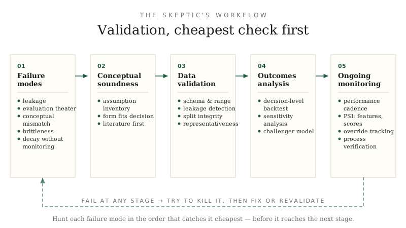
Figure — the skeptic’s workflow: hunt failure in the order that catches it cheapest, and try to kill the model at every stage.
And the mindset underneath all three: your job as validator is to kill the model, and the model only earns deployment by surviving. Confirmation metrics are cheap. The expensive, valuable evidence is the failure mode you went looking for and didn’t find — the subgroup where calibration holds, the challenger that loses honestly, the drift monitor that stays green through a population shift. Document the attempts, not just the successes: “we tried to break it here, here, and here; here’s what we found” is the most trustworthy sentence in any validation report.
A model that survives honest attempts at destruction is the only kind worth deploying. Everything else is a metric with good PR.