Companion repository: Poker-Chip-Simulation
The game and the question
The setup is a classroom game, simulated in Rockwell Arena (Student Edition): four participants, P1 through P4, arranged in a sequential workflow. Chips enter at P1 and each participant passes chips downstream according to the roll of a custom 8-sided die. When a participant doesn’t hold enough chips to satisfy a full roll, a partial batch moves instead — the classic starvation dynamic of any serial line.
The experimental question is concrete: which die configuration minimizes the work the last participant has to do — the number of P4 rolls required to push 100 chips through the system? Two candidate dice were tested:
- Team 1:
DISC(0.5, 2, 1.0, 8) - Team 2:
DISC(0.5, 1, 1.0, 9)
Each configuration ran 100 chips per replication, 120 replications each, with P4’s rolls counted via global tallying and the two configurations compared with a paired t-test at 90% confidence. The reported results: Team 1 averaged 1.30 P4 rolls (SD 0.18, CI ±0.03); Team 2 averaged 2.01 (SD 0.18, CI ±0.03).
A toy problem, but the experimental machinery around it — replications, pairing, and honest reporting — is exactly the machinery behind serious simulation studies. Here’s how to think about each piece.
(Note on the code in this article: the Python below is my own simplified reconstruction of the experiment’s statistical machinery — the replication loop, the pairing, the t-test — not a port of the Arena model. It replicates the analysis, not the simulation, so don’t compare its absolute numbers to the Arena results: the Arena model tallies P4 rolls under the classroom game’s exact turn rules, while this analog exists to demonstrate the pairing and the test.)
What DISC actually says
Arena’s DISC function takes cumulative-probability/value pairs and defines a discrete distribution. DISC(0.5, 2, 1.0, 8) means: with cumulative probability 0.5 the outcome is 2, and with cumulative probability 1.0 the outcome is 8. In plain terms:
- Team 1: P(X = 2) = 0.5, P(X = 8) = 0.5
- Team 2: P(X = 1) = 0.5, P(X = 9) = 0.5
Now compute the expected value of each die. Both are 5 chips per roll: (2+8)/2 = 5, (1+9)/2 = 5. The two dice have identical means. If you reasoned about this system with averages alone, you’d predict identical performance — and you’d be wrong by roughly 35%.
This is the first lesson the experiment teaches: the system is nonlinear, so the spread of the input distribution matters, not just its center. Team 2’s die has a heavier downside tail — a roll of 1 instead of 2. In a serial line with partial batches, small rolls are poison: they dribble chips downstream one at a time while everyone upstream waits, and they force more rolls per chip delivered. The variance interacts with the system’s starvation dynamics, and the mean can’t see it. Any time someone tells you “the average demand is the same, so the two policies are equivalent,” this is the counterexample to reach for.
Terminating simulations get replications — not one long run
The most common design error in simulation studies is running one long simulation and treating observations within it as independent samples. For this poker-chip game, that would be wrong for a structural reason: the simulation is terminating. It starts empty (no chips in the system) and ends at a natural event (100 chips have exited P4). There is no steady state to reach and no warm-up period to discard — the transient behavior is the behavior of interest, because a real run of the game always starts empty.
The correct design is independent replications: reset to the initial state, run to the terminating event, record one number (P4’s rolls), repeat 120 times. Each replication is an independent draw from the distribution of the performance measure, which means classical statistics apply directly — sample means, standard errors, t-intervals — with no batch-means machinery and no autocorrelation corrections.
This distinction generalizes. If you’re simulating a bank branch over one business day, a factory shift, or a disaster-response scenario, you have a terminating simulation: use replications. If you’re simulating a router running indefinitely, you have a steady-state simulation: use one long run (or a few) with warm-up deletion and batch means. Matching the statistical design to the simulation type is the step most often skipped, and it’s the step that determines whether your confidence intervals mean anything at all.
A note on the number 120: replication count is a precision decision. The standard error of the mean shrinks as 1/√n, so each additional replication buys less precision than the last. With SD 0.18 and n = 120, the standard error is 0.18/√120 ≈ 0.0164, and the 90% interval half-width is t₀.₀₅,₁₁₉ × 0.0164 ≈ 1.658 × 0.0164 ≈ 0.027 — which rounds to the reported ±0.03. The replication count was evidently chosen (or at least happens to deliver) a CI tight enough that the two configurations’ intervals don’t come close to touching. That’s what “enough replications” looks like: enough that the interval answers the question you actually asked.
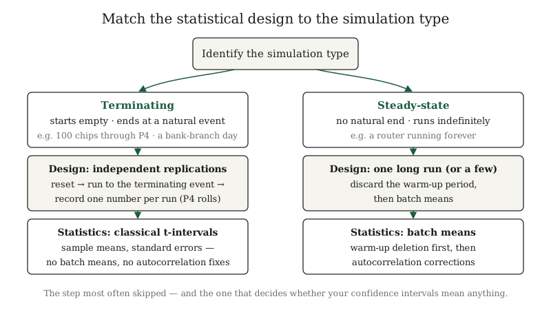
Figure — Match the statistical design to the simulation type: terminating simulations get independent replications, steady-state ones get long runs with warm-up deletion.
Paired comparisons: compare the dice, not the luck
The two die configurations weren’t run on independent random streams — they were compared with a paired t-test, which means each replication of Team 1 was matched with a replication of Team 2 under the same underlying randomness. This is the technique of common random numbers (CRN), and it’s the single highest-leverage variance-reduction trick in comparative simulation.
The intuition: suppose replication 7 happens to draw an unlucky sequence — long runs of small rolls. Both dice suffer it. When you take the difference between the two configurations on that replication, the shared bad luck cancels out. What’s left is the signal you care about: the systematic effect of the die itself.
The math makes the payoff precise. For the mean difference D̄ across n paired replications:
Var(D̄) = (σ₁² + σ₂² − 2ρσ₁σ₂) / n
where ρ is the correlation between the paired outcomes. With independent streams, ρ = 0 and you pay the full sum of both variances. With common random numbers, ρ > 0 — the same luck pushes both outcomes in the same direction — and the variance of the difference shrinks. In a well-paired comparison, most of the noise in the two arms is shared noise, so it subtracts away.
The clean way to implement CRN is not “use the same seed and hope the draws line up” — consumption order can drift between configurations. It’s the inverse-transform method on a shared uniform stream: generate one sequence of U(0,1) draws per replication, and map each draw through each policy’s own inverse CDF. Draw u = 0.3 maps to 2 under Team 1’s die and to 1 under Team 2’s die — same quantile, different outcome, perfectly synchronized randomness. The Python below does exactly this.
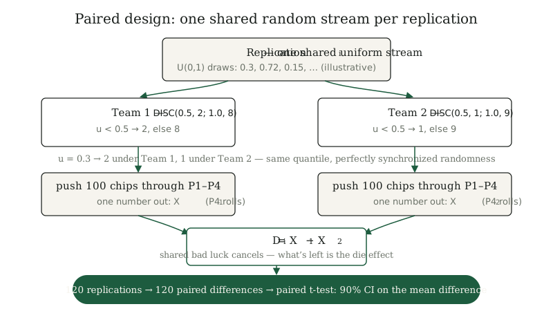
Figure — Paired design with common random numbers: one shared uniform stream per replication feeds both dice; the difference in P4 rolls is what gets tested.
A runnable version of the experiment
This is a simplified analog of the workflow — four stages in turn, each rolling its die and moving min(roll, available chips) downstream, P4’s rolls tallied until 100 chips exit — with the pairing implemented via a shared uniform stream:
import numpy as np
from scipy import stats

# Arena DISC(0.5, 2, 1.0, 8) -> P(X=2) = 0.5, P(X=8) = 0.5
# Arena DISC(0.5, 1, 1.0, 9) -> P(X=1) = 0.5, P(X=9) = 0.5
TEAM1 = (2, 8)
TEAM2 = (1, 9)

def replicate(uniforms, outcomes, target=100):
    """One replication: push `target` chips through P1..P4.

    `uniforms` is a shared U(0,1) stream (common random numbers); each
    policy maps the same draws through its own inverse CDF.
    Returns P4 rolls per chip delivered.
    """
    wip = [0, 0, 0]          # chips waiting between P1-P2, P2-P3, P3-P4
    delivered = 0
    p4_rolls = 0
    k, n = 0, len(uniforms)
    while delivered < target:
        for stage in range(4):                    # P1, P2, P3, P4 in turn
            u = uniforms[k % n]
            k += 1
            roll = outcomes[0] if u < 0.5 else outcomes[1]   # inverse CDF
            if stage == 0:
                moved = roll                      # P1 draws from supply
            else:
                moved = min(roll, wip[stage - 1])  # partial batch if starved
                wip[stage - 1] -= moved
            if stage < 3:
                wip[stage] += moved
            else:
                p4_rolls += 1
                delivered += moved
    return p4_rolls / target

def run_experiment(n_rep=120, seed=20260920):
    rng = np.random.default_rng(seed)
    t1 = np.empty(n_rep)
    t2 = np.empty(n_rep)
    for i in range(n_rep):
        uniforms = rng.random(4096)      # one stream, used by BOTH policies
        t1[i] = replicate(uniforms, TEAM1)
        t2[i] = replicate(uniforms, TEAM2)
    return t1, t2

t1, t2 = run_experiment()
d = t1 - t2                              # paired differences
n = len(d)
mean_d = d.mean()
se_d = d.std(ddof=1) / np.sqrt(n)
ci_low, ci_high = stats.t.interval(0.90, n - 1, loc=mean_d, scale=se_d)
res = stats.ttest_rel(t1, t2)            # paired t-test, same pairing

print(f"Team 1 mean rolls/chip: {t1.mean():.3f} (SD {t1.std(ddof=1):.3f})")
print(f"Team 2 mean rolls/chip: {t2.mean():.3f} (SD {t2.std(ddof=1):.3f})")
print(f"Paired difference: {mean_d:.3f}, 90% CI ({ci_low:.3f}, {ci_high:.3f})")
print(f"Paired t = {res.statistic:.2f}, p = {res.pvalue:.3g}")
print(f"Pairing correlation: {np.corrcoef(t1, t2)[0, 1]:.3f}")
Three things to notice in this code. First, the pairing is structural: the same uniforms array feeds both policies, so the correlation between arms is induced by construction — check the printed correlation to see CRN working. Second, ttest_rel tests the paired differences, which is the test the Arena study specified; an unpaired ttest_ind on the same data would be the wrong test for this design. Third, the interval that matters is the CI on the difference, not the two separate CIs — I’ll come back to why.
Read the interval, not the point — and report what’s actually missing
The reported results are means with intervals: 1.30 ± 0.03 versus 2.01 ± 0.03. Two observations follow, one statistical and one about honesty.
The statistical one: a gap of 0.71 between point estimates, with each mean’s standard error around 0.016, is enormous relative to the noise. Even under the conservative (unpaired) approximation, the implied t-statistic is on the order of 30 — the difference is not a sampling artifact. But the correct inference for a paired design is the interval on the paired difference, which the README does not report. Eyeballing whether two separate intervals overlap is a rough heuristic; the paired difference interval is the quantity the experiment was designed to produce.
The honesty one: the README documents the analysis setup — paired t-test at 90% confidence — but the p-value cell is empty. So here is what I will and won’t say. I will say the design is sound, the CIs are tight, and the gap dwarfs the sampling noise. I will not quote a p-value, and I will not write “the difference is statistically significant at α = 0.10” as if I’d seen the test output — because I haven’t, and neither has anyone reading that README. This is the discipline that separates engineering statistics from cargo-cult statistics: report the design you ran, the summaries you computed, and the exact cells that are empty. An empty cell is information. Filling it in from imagination is fabrication.
There’s a broader point hiding here about pre-registration. The study fixed its metric (P4 rolls), its design (paired), and its confidence level (90%) before running — that’s why the setup is worth describing even with the p-value missing. If you pick your test after seeing the data, no p-value means anything. Decide the analysis with the design, write it down, then run the replications.
How this generalizes to engineering practice
Strip away the poker chips and this is a template for any comparative simulation study:
- Identify the simulation type. Terminating (a shift, a mission, a batch of 100 units) → independent replications. Steady-state (a network running forever) → long runs with warm-up deletion. The statistics follow from this choice.
- Replicate enough to answer the question. Don’t pick n = 30 out of habit; pick n so the CI half-width is small relative to the difference you need to detect. The 1/√n rule lets you size a pilot run first, then scale.
- Pair your comparisons. When comparing policies, run them under common random numbers via shared uniform streams and inverse-transform sampling. It costs nothing and can cut the required replications severalfold.
- Report intervals, and report gaps. Means with CIs, the CI on the paired difference, the design (paired/unpaired, confidence level), and an explicit note of anything that didn’t get recorded. If a result is inconclusive — intervals overlapping, wide CI on the difference — say so, say how many more replications would settle it, and resist the urge to keep running until the answer looks nice. That last temptation has a name (optional stopping), and it invalidates the test.
The same habits transfer directly to A/B testing and capacity planning: a terminating simulation’s replications are the analog of randomized experimental units, CRN is the analog of blocking, and an honest CI is worth more than a significant-looking point estimate. The poker-chip game is small enough to hold in your head, which is exactly why it’s a good place to learn the discipline — the mistakes are cheap there, and the habits are portable everywhere else.